Tests

PAGE SCOPE

This page gives a set of synthetic data examples that act as functional and software tests, as well as indicating key performance characteristics in the areas of accuracy and resilience to data imperfections. Real data examples are given in the blog posts.

All figures on this page are actual outputs of the software, with synthetic data inputs. Synthetic station records generally have an identical “base” temperature history in a particular example, and also a common regional set of temperature fluctuations. Most examples have a separate, uncorrelated set of random temperature fluctuations, representing local variability, applied to each station record.

Example 01: Formation of Regional Averages

The following figure, showing synthetic monthly average temperature data, illustrates station raw data and their moving averages, and the separate formation of the monthly regional-averages of:

• moving average variations (relative to the arbitrary  reference year of 112)
• weather fluctuations relative to the moving averages

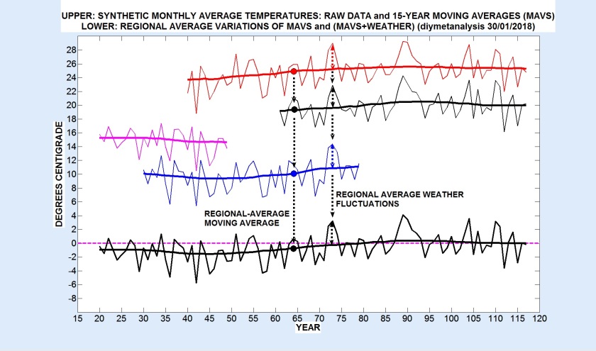
Note in the figure above that station moving averages extend right up to boundaries, see the Algorithms page for details of how this is done.

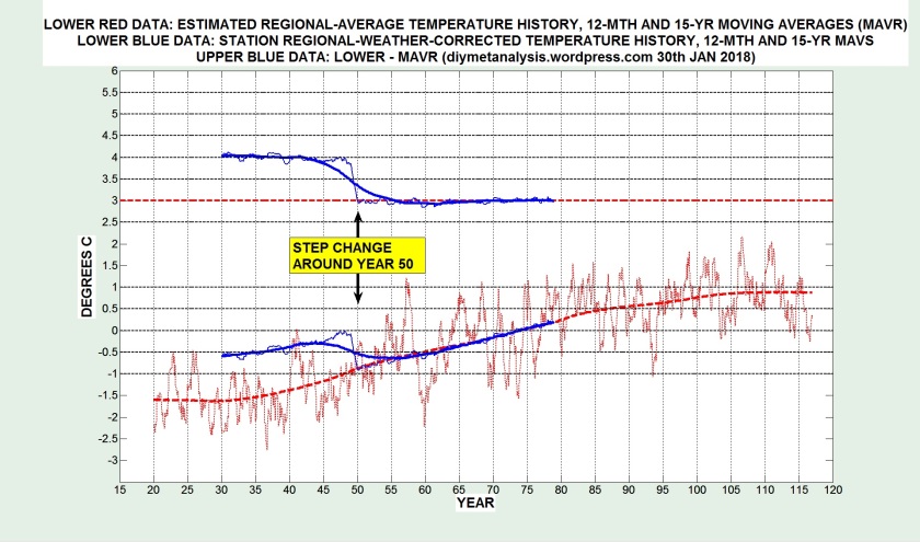
Example 02: Detection and Analysis of an Inhomogeneity

The following figure illustrates the main method of detecting inhomogeneities, the comparison of 12-month moving averages of regional-weather-corrected temperatures with the latest estimate of the regional moving averages (also plotted as a 12-month moving average):

The monthly data version of the figure above can often identify the date of step changes, sometimes with only a month or two of uncertainty:

 

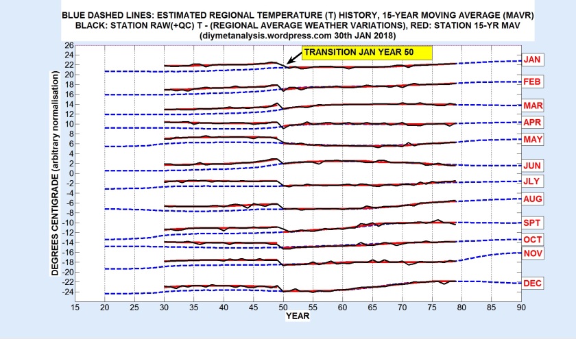
In the figure above the transition date of January of year 50 was recorded and used by the software, giving separate moving average periods (shown as the red curves) before and after the transition.

Example 03: Resilience to End-point Errors

The following figure shows synthetic monthly temperature data for 4 stations, one of which (the blue data) has a step change in temperature at year 50 (identified as a transition), together with a transient perturbation just before:

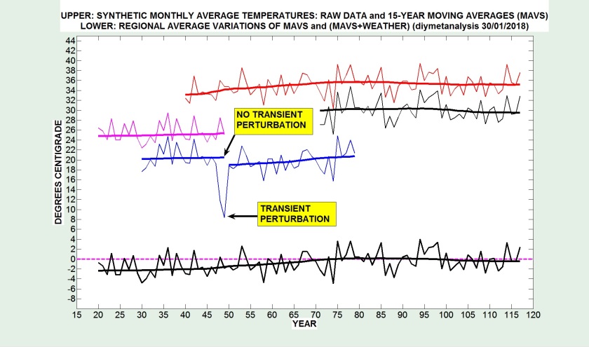
The purple data in the figure above is identical to the blue data up till the transient perturbation, which has negligible effect on both the station moving average and the regional average weather fluctuations.

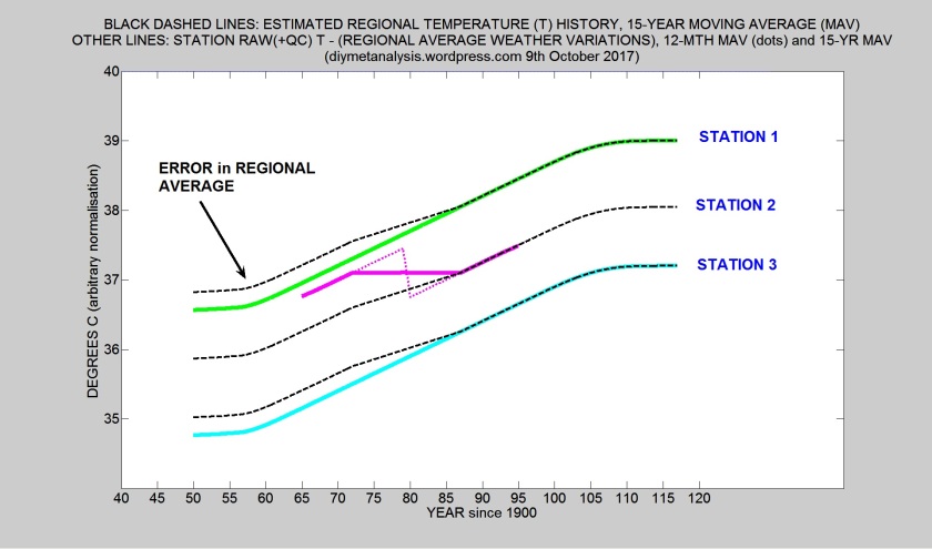
Example 04: Removing Transition Errors

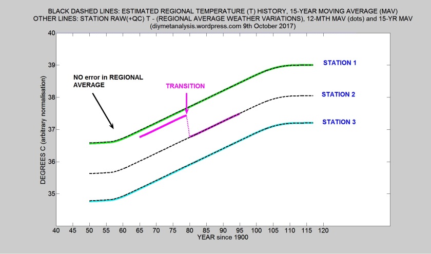
The following two figures show how errors caused by non-climatic changes in station-response are removed by manual detection and definition of “transitions”. The figure below shows a sudden anomalous shift in temperature in the purple data, causing an error in the regional moving average (in black):

The following figure shows that when a transition is defined the procedure deals correctly with the newly formed end points, removing the error in the regional moving average.

Example 05: Resilience to Transient Perturbations

The following figure was derived from a number of synthetic temperature records, one of which has a set of transient perturbations in its raw temperature data, similar in size to those seen in real data:

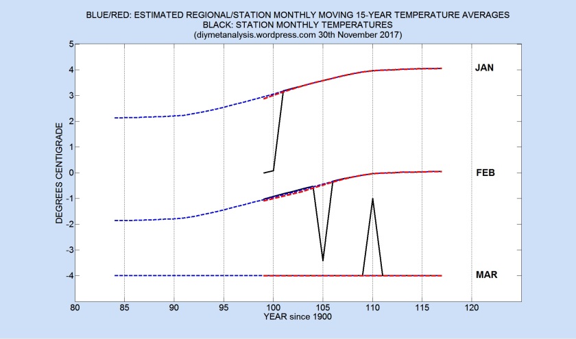
The figure above shows how the station (red) and regional (blue) moving averages are barely altered by the transient perturbations in the raw station temperature data (black). Most noteworthy is the lack of impact of the anomalous dip in temperatures at the start of the JAN data (the uppermost set of lines); such end-point anomalies make life difficult for methods based on interannual temperature changes. The moving-average algorithm used is resilient to, but not entirely unaffected by, end-point anomalies. Without such resilience the station and regional moving averages for the JAN data would be biased low before year 101.

Transient perturbations within (rather than at the ends of) temperature records are much less likely to give errors in the method, because any bias they create when the perturbation starts is usually removed when it ends, except when there is a change in the number of stations being averaged within the perturbation. The problem of time-varying station weights in the regional moving average makes it desirable to limit the influence of transient perturbations within records, a characteristic of the algorithm used to estimate moving averages, as explained in the Algorithms page.

END OF PAGE